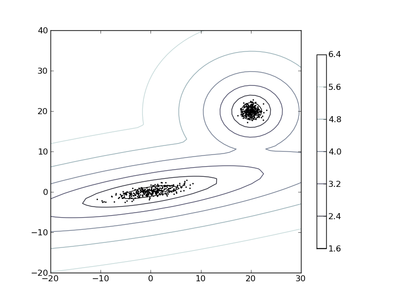
Density Estimation for a mixture of Gaussians

Plot the density estimation of a mixture of two gaussians. Data is generated from two gaussians with different centers and covariance matrices.

Python source code: plot_gmm_pdf.py

import numpy as np
import pylab as pl
from scikits.learn import mixture

n_samples = 300

# generate random sample, two components
np.random.seed(0)
C = np.array([[0., -0.7], [3.5, .7]])
X_train = np.r_[np.dot(np.random.randn(n_samples, 2), C),
          np.random.randn(n_samples, 2) + np.array([20, 20])]

clf = mixture.GMM(n_states=2, cvtype='full')
clf.fit(X_train)

x = np.linspace(-20.0, 30.0)
y = np.linspace(-20.0, 40.0)
X, Y = np.meshgrid(x, y)
XX = np.c_[X.ravel(), Y.ravel()]
Z =  np.log(-clf.eval(XX)[0])
Z = Z.reshape(X.shape)

CS = pl.contour(X, Y, Z)
CB = pl.colorbar(CS, shrink=0.8, extend='both')
pl.scatter(X_train[:, 0], X_train[:, 1], .8)

pl.axis('tight')
pl.show()