Generalized Linear Models
The following are a set of methods intended for regression in which
the target value is expected to be a linear combination of the input
variables. In mathematical notion, if  is the predicted
value.
is the predicted
value.

Across the module, we designate the vector  as coef_ and
  as intercept_.
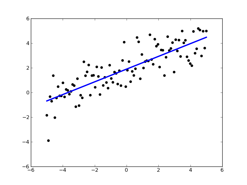
Ordinary Least Squares (OLS)
LinearRegression fits a linear model with coefficients
 to minimize the residual sum
of squares between the observed responses in the dataset, and the
responses predicted by the linear approximation.
to minimize the residual sum
of squares between the observed responses in the dataset, and the
responses predicted by the linear approximation.
LinearRegression will take in its fit method arrays X, y
and will store the coefficients  of the linear model in its
coef_ member.
of the linear model in its
coef_ member.
>>> from scikits.learn import glm
>>> clf = glm.LinearRegression()
>>> clf.fit ([[0, 0], [1, 1], [2, 2]], [0, 1, 2])
LinearRegression(fit_intercept=True)
>>> clf.coef_
array([ 0.5,  0.5])
However, coefficient estimates for Ordinary Least Squares rely on the
independence of the model terms. When terms are correlated and the
columns of the design matrix  have an approximate linear
dependence, the matrix
have an approximate linear
dependence, the matrix  becomes close to singular
and as a result, the least-squares estimate becomes highly sensitive
to random errors in the observed response, producing a large
variance. This situation of multicollinearity can arise, for
example, when data are collected without an experimental design.
becomes close to singular
and as a result, the least-squares estimate becomes highly sensitive
to random errors in the observed response, producing a large
variance. This situation of multicollinearity can arise, for
example, when data are collected without an experimental design.
Examples:
OLS Complexity
This method computes the least squares solution using a singular value
decomposition of X. If X is a matrix of size (n, p ) this method has a
cost of  , assuming that
  .
.
Ridge Regression
Ridge regression addresses some of the problems of Ordinary Least Squares (OLS) by imposing a penalty on the size of coefficients. The ridge coefficients minimize a penalized residual sum of squares,

Here,  is a complexity parameter that controls
the amount of shrinkage: the larger the value of
is a complexity parameter that controls
the amount of shrinkage: the larger the value of  , the
greater the amount of shrinkage.
, the
greater the amount of shrinkage.
>>> from scikits.learn import glm
>>> clf = glm.Ridge (alpha = .5)
>>> clf.fit ([[0, 0], [0, 0], [1, 1]], [0, .1, 1])
Ridge(alpha=0.5, fit_intercept=True)
>>> clf.coef_
array([ 0.34545455,  0.34545455])
>>> clf.intercept_
0.13636363636363638
Ridge Complexity
This method has the same order of complexity than an Ordinary Least Squares (OLS).
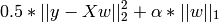
Lasso
The Lasso is a linear model trained with L1 prior as regularizer. The objective function to minimize is:
The lasso estimate thus solves the minimization of the
least-squares penalty with  added, where
is a constant and
added, where
is a constant and  is the L1-norm of the
parameter vector.
is the L1-norm of the
parameter vector.
This formulation is useful in some contexts due to its tendency to prefer solutions with fewer parameter values, effectively reducing the number of variables upon which the given solution is dependent. For this reason, the Lasso and its variants are fundamental to the field of compressed sensing.
This implementation uses coordinate descent as the algorithm to fit the coefficients. See LARS algorithm and its variants for another implementation.
>>> clf = glm.Lasso(alpha = 0.1)
>>> clf.fit ([[0, 0], [1, 1]], [0, 1])
Lasso(alpha=0.1, coef_=array([ 0.6,  0. ]), fit_intercept=True)
>>> clf.predict ([[1, 1]])
array([ 0.8])
The function lasso_path computes the coefficients along the full path of possible values.
Elastic Net
ElasticNet is a linear model trained with L1 and L2 prior as regularizer.
The objective function to minimize is in this case

LARS algorithm and its variants
Least-angle regression (LARS) is a regression algorithm for high-dimensional data, developed by Bradley Efron, Trevor Hastie, Iain Johnstone and Robert Tibshirani.
The advantages of LARS are:
- It is computationally just as fast as forward selection and has the same order of complexity as an ordinary least squares.
- It produces a full piecewise linear solution path, which is useful in cross-validation or similar attempts to tune the model.
- If two variables are almost equally correlated with the response, then their coefficients should increase at approximately the same rate. The algorithm thus behaves as intuition would expect, and also is more stable.
- It is easily modified to produce solutions for other estimators, like the Lasso.
- It is effective in contexts where p >> n (i.e., when the number of dimensions is significantly greater than the number of points)
The disadvantages of the LARS method include:
- Because LARS is based upon an iterative refitting of the residuals, it would appear to be especially sensitive to the effects of noise. This problem is discussed in detail by Weisberg in the discussion section of the Efron et al. (2004) Annals of Statistics article.
It is implemented using the LARS algorithm in class glm.LARS.
LARS Lasso
This implementation is based on the LARS algorithm, and unlike the implementation based on coordinate_descent, this yields the exact solution, which is piecewise linear as a function of the norm of its coefficients.
>>> from scikits.learn import glm
>>> clf = glm.LassoLARS(alpha=.1)
>>> clf.fit ([[0, 0], [1, 1]], [0, 1])
LassoLARS(max_features=None, alpha=0.1, normalize=True, fit_intercept=True)
>>> clf.coef_
array([ 0.50710678,  0.        ])
Getting the full path
See function scikits.learn.glm.lars_path:
- scikits.learn.glm.lars_path(X, y, Gram=None, max_features=None, alpha_min=0, method='lar', verbose=False)
Compute Least Angle Regression and LASSO path
Parameters : X: array, shape: (n, p) :
Input data
y: array, shape: (n) :
Input targets
max_features: integer, optional :
The number of selected features
Gram: array, shape: (p, p), optional :
Precomputed Gram matrix (X’ * X)
alpha_min: float, optional :
The minimum correlation along the path. It corresponds to the regularization parameter alpha parameter in the Lasso.
method: ‘lar’ or ‘lasso’ :
Specifies the problem solved: the LAR or its variant the LASSO-LARS that gives the solution of the LASSO problem for any regularization parameter.
Returns : alphas: array, shape: (k) :
The alphas along the path
active: array, shape (?) :
Indices of active variables at the end of the path.
coefs: array, shape (p,k) :
Coefficients along the path
Notes
Mathematical formulation
The algorithm is similar to forward stepwise regression, but instead of including variables at each step, the estimated parameters are increased in a direction equiangular to each one’s correlations with the residual.
Instead of giving a vector result, the LARS solution consists of a curve denoting the solution for each value of the L1 norm of the parameter vector. The full coeffients path is stored in the array coef_path_, which has size (n_features, max_features+1). The first column is always zero.
References:
- Original Algorithm is detailed in the paper Least Angle Regression by Hastie et al.
Bayesian Regression
Bayesian regression techniques can be used to include regularization
parameters in the estimation procedure. This can be done by
introducing some prior knowledge over the parameters. For example,
penalization by weighted  norm is equivalent to
setting Gaussian priors on the weights.
norm is equivalent to
setting Gaussian priors on the weights.
The advantages of Bayesian Regression are:
- It adapts to the data at hand.
- It can be used to include regularization parameters in the estimation procedure.
The disadvantages of Bayesian Regression include:
- Inference of the model can be time consuming.
Bayesian Ridge Regression
BayesianRidge tries to avoid the overfit issue of
Ordinary Least Squares (OLS), by adding the following prior on
 :
:
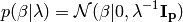
The resulting model is called Bayesian Ridge Regression, it is
similar to the classical Ridge.  is an
hyper-parameter and the prior over performs a
shrinkage or regularization, by constraining the values of the weights
to be small. Indeed, with a large value of , the
Gaussian is narrowed around 0 which does not allow large values of
, and with low value of , the Gaussian is
very flattened which allows values of . Here, we use a
non-informative prior for .
The parameters are estimated by maximizing the marginal log likelihood.
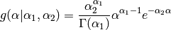
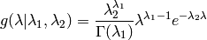
There is also a Gamma prior for and :
is an
hyper-parameter and the prior over performs a
shrinkage or regularization, by constraining the values of the weights
to be small. Indeed, with a large value of , the
Gaussian is narrowed around 0 which does not allow large values of
, and with low value of , the Gaussian is
very flattened which allows values of . Here, we use a
non-informative prior for .
The parameters are estimated by maximizing the marginal log likelihood.
There is also a Gamma prior for and :
- By default
 , i.e.
 - very slightly informative priors.
Bayesian Ridge Regression is used for regression:
>>> from scikits.learn import glm
>>> X = [[0., 0.], [1., 1.], [2., 2.], [3., 3.]]
>>> Y = [0., 1., 2., 3.]
>>> clf = glm.BayesianRidge()
>>> clf.fit (X, Y)
BayesianRidge(n_iter=300, verbose=False, lambda_1=1e-06, lambda_2=1e-06,
       fit_intercept=True, eps=0.001, alpha_2=1e-06, alpha_1=1e-06,
       compute_score=False)
After being fitted, the model can then be used to predict new values:
>>> clf.predict ([[1, 0.]])
array([ 0.50000013])
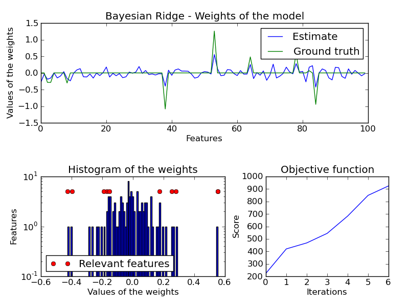
The weights of the model can be access:
>>> clf.coef_
array([ 0.49999993,  0.49999993])
Due to the Bayesian framework, the weights found are slightly different to the ones found by Ordinary Least Squares (OLS). However, Bayesian Ridge Regression is more robust to ill-posed problem.
Examples:
References
- More details can be found in the article paper by MacKay, David J. C.
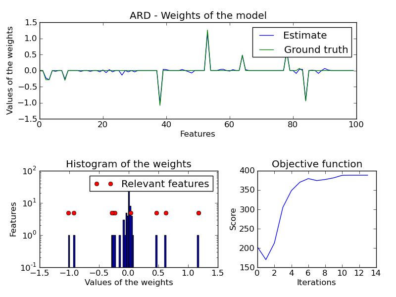
Automatic Relevance Determination - ARD
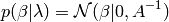
ARDRegression adds a more sophisticated prior ,
where we assume that each weight  is drawn in a
Gaussian distribution, centered on zero and with a precision
is drawn in a
Gaussian distribution, centered on zero and with a precision
 :
:
with  .
There is also a Gamma prior for and :
.
There is also a Gamma prior for and :
- By default , i.e.
- very slightly informative priors.
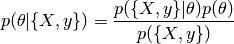
Mathematical formulation
A prior is introduced as a distribution  over the parameters.
This distribution is set before processing the data. The parameters of a prior
distribution are called hyper-parameters. This description is based on the
Bayes theorem :
over the parameters.
This distribution is set before processing the data. The parameters of a prior
distribution are called hyper-parameters. This description is based on the
Bayes theorem :
- With :
 the likelihood : it expresses how probable it is
to observe
the likelihood : it expresses how probable it is
to observe  given
given  .
. the marginal probability of the data : it can be
considered as a normalizing constant, and is computed by integrating
with respect to .
the marginal probability of the data : it can be
considered as a normalizing constant, and is computed by integrating
with respect to .- the prior over the parameters : it expresses the
knowledge that we can have about before processing the
data.
 the conditional probability (or posterior
probability) : it expresses the uncertainty in after
observing the data.
the conditional probability (or posterior
probability) : it expresses the uncertainty in after
observing the data.
All the following regressions are based on the following Gaussian assumption:

where is the precision of the noise.
References
- Original Algorithm is detailed in the book Bayesian learning for neural networks by Radford M. Neal