Clustering
Clustering of unlabeled data can be performed with the module scikits.learn.cluster.
This page contents:
Affinity propagation

- class scikits.learn.cluster.AffinityPropagation(damping=0.5, maxit=200, convit=30, copy=True)
Perform Affinity Propagation Clustering of data
Parameters : damping : float, optional
Damping factor
maxit : int, optional
Maximum number of iterations
convit : int, optional
Number of iterations with no change in the number of estimated clusters that stops the convergence.
copy: boolean, optional :
Make a copy of input data. True by default.
Notes
See examples/plot_affinity_propagation.py for an example.
Reference:
Brendan J. Frey and Delbert Dueck, “Clustering by Passing Messages Between Data Points”, Science Feb. 2007
The algorithmic complexity of affinity propagation is quadratic in the number of points.
Attributes
cluster_centers_indices_ array, [n_clusters] Indices of cluster centers labels_ array, [n_samples] Labels of each point Methods
fit: Compute the clustering - fit(S, p=None, **params)
compute MeanShift
Parameters : S: array [n_points, n_points] :
Matrix of similarities between points
p: array [n_points,] or float, optional :
Preferences for each point
damping : float, optional
Damping factor
copy: boolean, optional :
If copy is False, the affinity matrix is modified inplace by the algorithm, for memory efficiency
Examples:
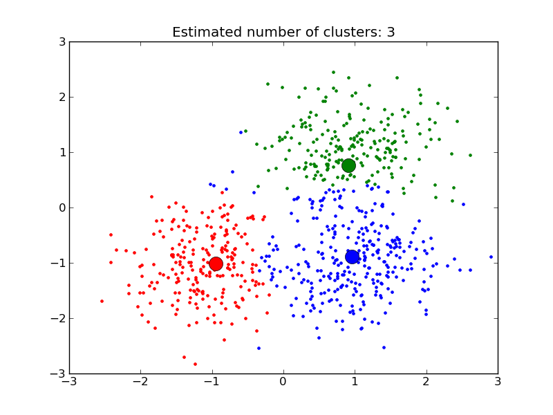
- example_plot_affinity_propagation.py: Affinity Propagation on a synthetic 2D datasets with 3 classes.
- Finding structure in the stock market Affinity Propagation on Financial time series to find groups of companies
Mean Shift
- class scikits.learn.cluster.MeanShift(bandwidth=None)
MeanShift clustering
Parameters : bandwidth: float, optional :
Bandwith used in the RBF kernel If not set, the bandwidth is estimated. See clustering.estimate_bandwidth
Notes
Reference:
K. Funkunaga and L.D. Hosteler, “The Estimation of the Gradient of a Density Function, with Applications in Pattern Recognition”
The algorithmic complexity of the mean shift algorithm is O(T n^2) with n the number of samples and T the number of iterations. It is not adviced for a large number of samples.
Attributes
cluster_centers_: array, [n_clusters, n_features] Coordinates of cluster centers labels_: Labels of each point Methods
fit(X): Compute MeanShift clustering - fit(X, **params)
Compute MeanShift
Parameters : X : array [n_samples, n_features]
Input points
Examples:
- example_plot_mean_shift.py: Mean Shift clustering on a synthetic 2D datasets with 3 classes.
K-means
- class scikits.learn.cluster.KMeans(k=8, init='random', n_init=10, max_iter=300)
K-Means clustering
Parameters : data : ndarray
A M by N array of M observations in N dimensions or a length M array of M one-dimensional observations.
k : int or ndarray
The number of clusters to form as well as the number of centroids to generate. If init initialization string is ‘matrix’, or if a ndarray is given instead, it is interpreted as initial cluster to use instead.
n_iter : int
Number of iterations of the k-means algrithm to run. Note that this differs in meaning from the iters parameter to the kmeans function.
init : {‘k-means++’, ‘random’, ‘points’, ‘matrix’}
Method for initialization, defaults to ‘k-means++’:
‘k-means++’ : selects initial cluster centers for k-mean clustering in a smart way to speed up convergence. See section Notes in k_init for more details.
‘random’: generate k centroids from a Gaussian with mean and variance estimated from the data.
‘points’: choose k observations (rows) at random from data for the initial centroids.
‘matrix’: interpret the k parameter as a k by M (or length k array for one-dimensional data) array of initial centroids.
Notes
The k-means problem is solved using the Lloyd algorithm.
The average complexity is given by O(k n T), were n is the number of samples and T is the number of iteration.
The worst case complexity is given by O(n^(k+2/p)) with n = n_samples, p = n_features. (D. Arthur and S. Vassilvitskii, ‘How slow is the k-means method?’ SoCG2006)
In practice, the K-means algorithm is very fast (on of the fastest clustering algorithms available), but it falls in local minimas, and it can be useful to restarts it several times.
Attributes
cluster_centers_: array, [n_clusters, n_features] Coordinates of cluster centers labels_: Labels of each point inertia_: float The value of the inertia criterion associated with the chosen partition. Methods
fit(X): Compute K-Means clustering - fit(X, **params)
Compute k-means
Spectral clustering
Spectral clustering is especially efficient if the affinity matrix is sparse.
- class scikits.learn.cluster.SpectralClustering(k=8, mode=None)
Spectral clustering: apply k-means to a projection of the graph laplacian, finds normalized graph cuts.
Parameters : k: integer, optional :
The dimension of the projection subspace.
mode: {None, ‘arpack’ or ‘amg’} :
The eigenvalue decomposition strategy to use. AMG (Algebraic MultiGrid) is much faster, but requires pyamg to be installed.
Attributes
labels_: Labels of each point Methods
fit(X): Compute spectral clustering - fit(X, **params)
Compute the spectral clustering from the adjacency matrix of the graph.
Parameters : X: array-like or sparse matrix, shape: (p, p) :
The adjacency matrix of the graph to embed.
Notes
If the pyamg package is installed, it is used. This greatly speeds up computation.
Examples:
- Segmenting the picture of Lena in regions: Spectral clustering to split the image of lena in regions.
- Spectral clustering for image segmentation: Segmenting objects from a noisy background using spectral clustering.